R function: block average
R ·Commonly, we need to calculate a mean value of a sequence of numbers, and we would also calculate a level of uncertainty for that estimate. This is, the standard error, which is calculated as the quotient between the standard deviation of the data and the squared root of the number of observations.
However, this procedure turns out to be wrong when our data is not independent. This is the case, for example, of time series data: each new value of the sequence depends more or less of the values recorded previously.
The block average method
Calculating the standard error of not independent data by using the classic equation would output very artificially small standard errors for the mean. Although we have n samples, these are not independent (for example, in the case of time series), so in reality we have a less number of independent samples. The block average method is useful to deal with this problem. This method consists on dividing the data (N values) in n chunks or blocks of equal size s (n * s = N). Then, we compute the mean value for each block, the mean of these block means, and the standard error for the latter (the mean of means).
Then, the key of the method consists on determining the “correct” size of the blocks, from which the blocks of data are independent from each other. A good way to do this consists on calculating the standard error of the mean of means (means in plural, for each calculated mean per block of a fixed size), for different values of block sizes. Then, plotting these estimates in relation to the the size of the blocks. The best value of the standard error would be the one that remains more or less constant while the size of the blocks increases.
For this purpose, I have coded an R function. Let’s see an example that hopefully will clarify the method.
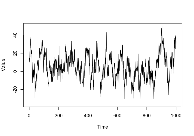
Firstly, we simulate some random and non-independent data. We will simulate a time series:
# We set the seed in order to get always the same results
set.seed(42)

# Generates 1000 random values from a normal distribution
# with mean = 1 and sd = 10
x <- rnorm(1000, mean = 1, sd = 10)

# We generate a new variable "sum" that will be calculated as the sum
# of the actual value, plus the three previous values premultiplied by
# a random coefficiente
sum <- rep(0, length(x))
sum[1] <- x[1]
for(i in 2:length(x))
{
  # Do the work only if there are three values down
  if(i > 3)
  {
    sum[i] <- runif(1, 0.5, 1) * x[i] + runif(1, 0.4, 0.6) * sum[i-1] +
              runif(1, 0.2, 0.4) * sum[i-2] + runif(1, 0, 0.2) * sum[i-3]
  }
  else
  {
    sum[i] <- sum[i-1] + x[i]
  }
}
Let’s see how the plot of this simulated time series look likes:
Then, we apply the block average method, by using the function block_average in R. This functions has three arguments: x is the sequence of numbers (a numeric vector) from which we want to calculate a standard error; block_sizes is a numeric vector which contains the different block sizes to be assessed; and n_blocks is a numeric vector with the number of blocks to be evaluated. The two latter arguments are optional, although is recommended to define one of them. If n_blocks is defined, the sizes of the blocks to be evaluated are automatically calculated. For instance, let’s imagine we have a sequence of 100 numbers from a time series, and we define n_blocks = c(10, 25, 50). Then, the sizes of the blocks will be calculated as 100 (the length of the numeric sequence) divided by each number of n_blocks: 10, 4, and 2. If both arguments are defined, the function only works with the values defined on block_sizes. I recommend to manually define the block sizes in the block_sizesargument, as it is more intuitive.
The function outputs a scatter plot with the standard errors in relation to the block size. If assigned to a object, the function also returns a dataframe from which the plot is created. This may be useful if the user wants to do some extra analyses. In our example:
# seq(5, 150, 5) defines a sequence of numbers from 5 to 150, by 5
block_average(x = sum, block_sizes = seq(5, 150, 5))
The plot:
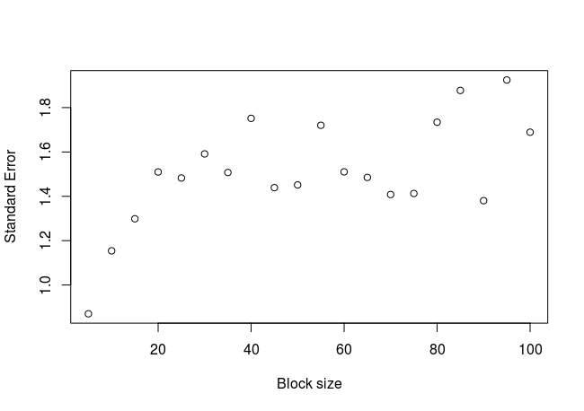
We can see that the standard error increases in a logarithmic way, until a value of approximately 1.6 from which the trend appears to stabilize. We could fit a curve to this cloud of points, in order to get a more precise value of the stabilized standard error (not done here). What happens if we calculate the standard error in the classic way?
sd(sum) / sqrt(length(sum))
>> 0.4302361
As expected, the standard error calculated with the block average method is larger than the one calculated classically. This happens because the number of real independent samples are less than the total number of samples.
What happens if we apply the block average method to an independent set of numbers? In the simulated sequence above, the vector x contains independent numbers. Let’s apply the function to this vector:
block_average(x = x, block_sizes = seq(5, 150, 5))
The plot:
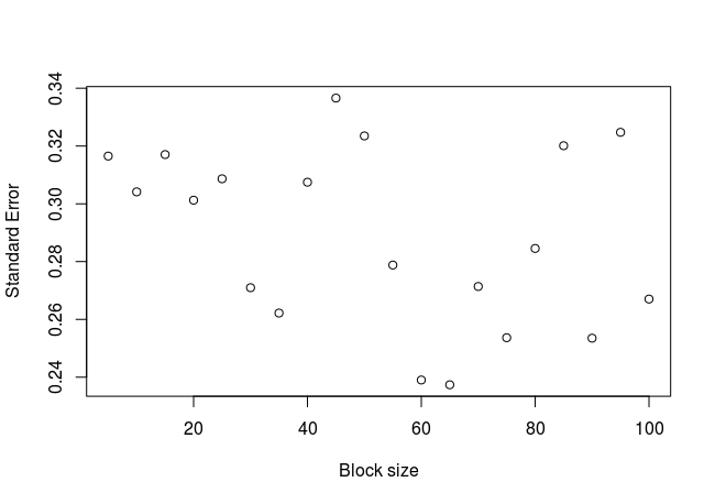
As expected, there is no clear relationship between the standard error and the block size for independent values.
Here are some references of the block average method:
http://sachinashanbhag.blogspot.com/2013/08/block-averaging-estimating-uncertainty.html
https://www.quora.com/What-is-the-block-average-method
http://realerthinks.com/block-averaging-bootstrapping-estimating-mean-autocorrelated-data/
You can get the full code for this function from my GitHub page, here.